Boundary conditions (in-plane)

Discrete boundary

The continuous boundary, as defined by the equilibrium, typically does not align with the boundary points of the mesh, where boundary conditions are applied in PARALLAX. Consequently, the discrete boundary approximates the continuous boundary in a step-wise fashion. If boundary information is only available on the continuous boundary, this approximation can reduce numerical accuracy and consistency, especially for Neumann boundary conditions. However, in most practical applications, the in-plane boundary conditions are usually surrounded by non-physical buffer zones, and the boundary conditions (such as Dirichlet or homogeneous Neumann) are not overly complex. As a result, this approach seems generally sufficient for a wide range of use cases.

Neumann boundary conditions

For the treatment of Neuman boundary conditions, we define a discrete normal direction spanned by the polygon running along the boundary points. To do so, we first introduce a discrete level set function defined as follows: $$\begin{align} \Psi_{i,j} = \begin{cases}1 \quad \text{for inner grid point} \\ \frac{1}{2} \quad \text{for boundary point} \\ 0 \quad \text{otherwise}\end{cases}. \end{align}$$ Note that $\Psi$ is also defined for ghost points and points where no grid point is present. Next, for each boundary point, we define the discrete normal direction as: $$\begin{align} \mathbf{n}_{i,j} =\left(\Psi_{i+1,j}-\Psi_{i-1,j},\,\Psi_{i,j+1}-\Psi_{i,j-1}\right)^T. \end{align}$$ This normal is generally not normalized and its components $nx_{i,j}, ny_{i,j}$ can take values of $[-1, -\dfrac{1}{2}, 0, \dfrac{1}{2}, 1]$.

To define the discrete normal gradient, we compute the upstream value of a given variable $u$ at a boundary point as follows: $$\begin{align} u_{i,j}^N = u_{i+nx_{i,j},j+ny_{i,j}}, \end{align}$$ provided that both $nx_{i,j}, ny_{i,j}$​ are integer values. If $nx_{i,j}$​ is an integer and $ny_{i,j}$​ is a half-integer, we modify the computation to: $$\begin{align} u^N_{i,j} = \frac{1}{2}u_{i+nx_{i,j},j}+\frac{1}{2}u_{i+nx_{i,j},j+2ny_{i,j}}. \end{align}$$ Other cases involving $nx_{i,j}, ny_{i,j}$ ​ are handled similarly.

The discrete normal gradient is then computed as: $$\begin{align} \mathbf{n}\cdot\nabla u \rightarrow \frac{u^N_{i,j}-u_{i,j}}{h\sqrt{nx_{i,j}^2+ny_{i,j}^2}}. \end{align}$$

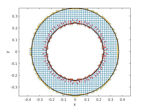
Example of discrete boundaries. The continuous boundary (black) is approximated by discrete polygons (red and orange). The red arrows represent the scaled normal vectors at the boundary points of the inner boundary.

Example: Setting Boundary Conditions

The following example demonstrates how to apply homogeneous Neumann boundary conditions at the core and Dirichlet boundary conditions with a value of 2 at the other boundaries for the dynamical variable $u$:

use descriptors_m, only : DISTRICT_..., BND_TYPE_NEUMANN, BND_TYPE_DIRICHLET_ZERO
use boundaries_perp_m, only : set_perpbnds
..
real(FP), dimension(mesh%get_n_points()) :: u ! This is the dynamical variable
integer, dimension(mesh%get_n_points_boundary()) :: bnd_descrs
real(FP), dimension(mesh%get_n_points_boundary()) :: bnd_vals
...
do kb = 1, mesh%get_n_points_boundary()
    l = mesh%boundary_indices(kb)
    district = mesh%get_district(l)
    select case(district)
        case(DISTRICT_CORE)
            bnd_descrs(kb) = BND_TYPE_NEUMANN
            bnd_vals(kb) = 0.0_FP
        case(DISTRICT_WALL, DISTRICT_PRIVFLUX, DISTRICT_DOME, DISTRICT_OUT)
            bnd_descrs(kb) = BND_TYPE_DIRICHLET_ZERO
            bnd_vals(kb) = 2.0_FP
        case default
            ! You can add error handling here, as boundary points must belong to one of the above districts
    end select
enddo

! Apply boundary conditions using the set_perpbnds function
call set_perpbnds(mesh, bnd_types, u, bnd_vals)
! The variable 'u' is returned with the values at the boundary points modified to satisfy the specified boundary conditions

In principle, a different boundary condition type and value can be specified for each boundary point. The type of boundary condition is chosen using the descriptors BND_TYPE_NEUMANN and BND_TYPE_DIRICHLET_ZERO. It is important to note that the _ZERO in the BND_TYPE_DIRICHLET_ZERO descriptor does not imply homogeneous Dirichlet boundary conditions, but is a historical artifact that remains for backward compatibility.