Polar mesh and operators

Motivation and disclaimer

For diagnostic purposes and certain specific applications, such as modeling sources or implementing zonal Neumann boundary conditions, the use of a polar mesh and associated operators can be highly beneficial. This mesh is not designed to advance variables on in time, but rather serves as an auxiliary feature provided by PARALLAX.

Certain functionalities of the polar module for 3D equilibria are still under development. While the coordinate mapping and polar mesh appear to be functioning correctly, the computation of the metric tensor currently assumes axisymmetry. As a result, flux surface averaging calculations may yield inaccurate results.

Polar coordinates

We define the transformation from cylindrical to polar coordinates as follows: $$\begin{align} \rho = &\rho(R, \varphi, Z), \\ \theta = & \arctan\left(\frac{Z}{R-R_0}\right) \\ \varphi = & \varphi, \end{align}$$ where $\rho$ represents the flux surface label provided by the equilibrium, and $\theta$ is the geometric poloidal angle. For diverted geometries, the normalized poloidal flux is commonly used: $$\begin{align} \rho = \sqrt{\frac{\Psi(R,Z)-\Psi_{0}}{\Psi_{X}-\Psi_{0}}} \end{align}$$ where $\Psi_0$ is the poloidal magnetic flux at the magnetic axis, and $\Psi_X$ is the poloidal flux at the separatrix. The polar coordinate system is defined only on closed magnetic flux surfaces, as its definition in open field-line regions could be ambiguous, especially in diverted geometries. PARALLAX provides routines for mapping coordinates between cylindrical and polar systems, as well as for calculating the associated metric tensor components $g^{\rho\rho}, g^{\rho\theta}, g^{\theta\theta}, g^{\varphi\varphi}$.

Polar grid

The polar grid is structured logically as a Cartesian and equidistant grid, defined as follows: $$\begin{align} \rho_{m} = &\rho_{min}+\Delta\rho (m-1),\quad m = 1,2,\dots n_\rho, \\ \theta_{n} = &\Delta\theta (n-1),\quad n = 1,2,\dots n_\theta. \end{align}$$ In the toroidal direction, the familiar poloidal planes are used indexed by $\varphi_k$​. The polar mesh for each plane individually can be initialized with the following call:

call polar_grid%initialize(equi, phi, nrho, ntheta)

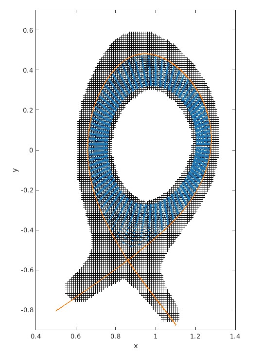
Polar grid (blue) defined on the closed field line region, with the Cartesian mesh shown as black crosses. The separatrix (orange) is shown for reference and not part of the polar mesh.

Mapping to polar grid

For mapping a field $u$ from the mesh to the polar grid the same interpolation method as used for the FCI mapping. The map operation can be written again via a sparse matrix, which has dimensions $n_\rho n_\theta \times n_{mesh}$, where $n_{mesh}$ is the number of mesh points per plane. The following code snippet illustrates how a map matrix is created and how a field is mapped to the polar grid on an individual plane.

! Interpolation order
intorder = 3
! Field on Cartesian mesh
real(FP), dimension(mesh%get_n_points()) :: u
! Field mapped to polar mesh (note the order of dimensions) 
real(FP), dimension(polar_grid%get_ntheta(), polar_grid%get_nrho()) :: upol
! Polar map matrix
type(csrmat_t) :: polar_map_csr

! Create polar map matrix
create_polar_map_matrix(polar_map_csr, equi, mesh, polar_grid, intorder)

! Map via sparse Matrix vector multiplication
call csr_times_vec(polar_map_csr, u, upol)

Flux surface operations

PARALLAX provides functionality to compute the flux surface average, which is essentially a volume average defined as (see here): $$\begin{align} \left\langle u \right\rangle = \lim_{V \to 0} \frac{1}{V} \int_V u \, dV, \end{align}$$ where $V$ is the closed volume between two flux surfaces. This expression can be rewritten in a more convenient form as: $$\begin{align} \left\langle u \right\rangle = \frac{\int_0^{2\pi} \int_0^{2\pi} u J \, d\theta \, d\varphi}{\int_0^{2\pi} \int_0^{2\pi} J \, d\theta \, d\varphi}, \end{align}$$ where $J$ is the Jacobian of the polar coordinate system.

For each plane, a sparse matrix of dimension $n_\rho \times n_{mesh}$ is constructed from the polar map matrix. To compute the flux surface average, the toroidal averaging step must still be performed explicitly, as shown in the following code:

! Field on Cartesian mesh
real(FP), dimension(mesh%get_n_points()) :: u
! Polar grid
type(polar_grid_t) :: polar_grid
! Polar map matrix (see above)
type(csrmat_t) :: polar_map_csr
! Flux surface average matrix
type(csrmat_t) :: fsa_csr
! Field on Cartesian mesh
real(FP), dimension(polar_grid%get_nrho()) :: u_fsa

! Create flux surface average matrix
call create_flux_surface_average_csr(fsa_csr, equi, mesh, &
                                      polar_grid, polar_map_csr)

! Compute flux surface average for a single plane
call csr_times_vec(fsa_csr, u, u_fsa)

! Perform toroidal average (=MPI-average)
call MPI_comm_size(MPI_COMM_WORLD, nprocs, ierr)

call MPI_allreduce(MPI_IN_PLACE, u_fsa, polar_grid%get_nrho(), &
                   MPI_GP, MPI_SUM, MPI_COMM_WORLD, ierr)

do ip = 1, polar_grid%get_nrho()
    u_fsa(ip) = u_fsa(ip) / nprocs
end do

In addition to the flux surface average, PARALLAX also supports the computation of surface averages, which are necessary for tasks such as calculating radial fluxes. To compute a surface average, use the routine call create_surface_average_csr to construct the corresponding sparse matrix. Otherwise, the procedure for surface averaging follows the same approach as the flux surface average.