More on parallel gradient

Motivation

Here, we present an advanced method for discretizing the parallel gradient, based on a coordinate-free representation, where areas are mapped instead of individual points. Therefore, this approach is more intuitive and performs better in situations with significant map distortions. The scheme was firstly introduced in A. Stegmeir et al., Comput Phys. Commun. 213:111, (2017), where you can also find verifications and illustrative examples.

Coordinate free represenatation

We start with the coordinate free representation of the parallel gradient: $$\begin{align} \nabla_\parallel u = \frac{1}{B}\nabla\cdot\left(\mathbf{B}u\right)=\frac{1}{B}\lim_{w\rightarrow 0}\frac{1}{\Omega_w}\int\limits_{\partial\Omega_w}u\mathbf{B}\cdot d\mathbf{S}, \end{align}$$ where $\Omega_w$ is an arbitrary volume parametrisation which continuously shrinks to zero with $w$, i.e. $\lim_{w\rightarrow 0}\Omega_w = 0$.

For clarity and compact notation in the following, we introduce the staggered grid index $\kappa=k+\frac{1}{2}$. We mimic the expression on the discrete level according to the sketch illustrated in the figure below: $$\begin{align} q_{i,j,\kappa}=\frac{1}{(BV)_{i,j,\kappa}}\left[\int_{A^+_{i,j,\kappa}}u_{k+1}B_{tor}dA - \int_{A^-_{i,j,\kappa}}u_{k}B_{tor}dA\right], \label{pargrad} \end{align}$$ where we choose the finite flux box volumes $\Omega_w$​ such that only the surface integrals at the toroidal ends remain. These surface integrals are retained on the continuous level within the poloidal planes $k$ and $k+1$.

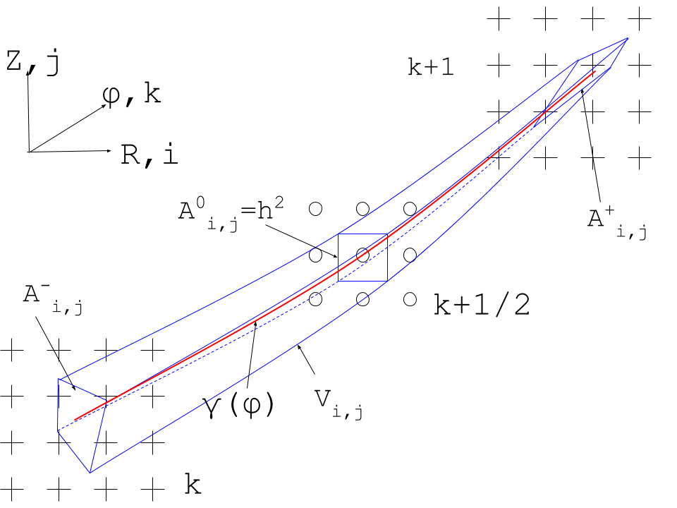
Sketch of the integration scheme for the parallel gradient: Blue represents the finite flux box being integrated, and red indicates the central field line.

Prefactor in eq. ($\ref{pargrad}$):

The pre-factor in eq. ($\ref{pargrad}$) is defined as $$\begin{align} (BV)_{i,j,\kappa} = \int\limits_{\varphi_\kappa-\frac{\Delta\varphi}{2}}^{\varphi_\kappa+\frac{\Delta\varphi}{2}} B(\mathbf{\gamma}(\varphi))\,A_c(\mathbf{\gamma}(\varphi))\,\gamma_R(\varphi)\,d\varphi, \end{align}$$ where $A_c$ represents the cross-sectional area of the flux box. This expression can be simplified by the fact that magnetic flux is conserved, and therefore: $$\begin{align} A_c(\gamma(\varphi))B_{tor}(\gamma(\varphi)) = const. = A_c(\gamma(\varphi_\kappa))B_{tor}(\gamma(\varphi_\kappa)) = h^2 B_{tor,i,j,\kappa}. \label{flux_cosnervation} \end{align}$$ This leads to: $$\begin{align} (BV)_{i,j,\kappa} = B_{tor,i,j,\kappa}h^2\int\limits_{\varphi_\kappa-\frac{\Delta\varphi}{2}}^{\varphi_\kappa+\frac{\Delta\varphi}{2}}\frac{B(\mathbf{\gamma}(\varphi))}{B_{tor}(\mathbf{\gamma}(\varphi))}\gamma_R(\varphi)\,d\varphi = B_{tor,i,j,\kappa}h^2 \left(s_{i,j,\kappa}\left(\frac{\Delta\varphi}{2}\right)+s_{i,j,\kappa}\left(-\frac{\Delta\varphi}{2}\right)\right). \end{align}$$ Therefore, the prefactor can be easily computed from the magnetic field line length along the central chord of the flux box (see field line tracing).

Quadrature in eq. ($\ref{pargrad}$):

Finally, we need to numerically integrate the surface terms in equation ($\ref{pargrad}$), which are located within the poloidal planes. To achieve this, we divide the area of interest into $2^X\times 2^X$ subcells or quadrature points, where (X \ge 0) is an integer parameter, and $s,t$ are the subcell indices (see figure below): $$\begin{align} \int_{A^\pm_{i,j,\kappa}}u_{\kappa\pm\frac{1}{2}}B_{tor}dA = \frac{h^2}{2^{2X}}\sum_{s,t=1}^{2^X}u_{\kappa\pm\frac{1}{2}}(R^\pm_{{(i,j,\kappa)}_s},\, Z^\pm_{{(i,j,\kappa)}_t})B_{tor}(R_{{(i,j,\kappa)}_s},\, Z_{{(i,j,\kappa)}_t}), \end{align}$$ where $$\begin{align} R_{{(i,j,\kappa)}_s} = R_{i,\kappa}-\frac{h}{2}+\frac{h}{2^X}\left(s-\frac{1}{2}\right), \\ Z_{{(i,j,\kappa)}_t} = Z_{j,\kappa}-\frac{h}{2}+\frac{h}{2^X}\left(t-\frac{1}{2}\right), \\ \text{and}\quad R^\pm_{{(i,j,\kappa)}_s},\,Z^\pm_{{(i,j,\kappa)}_t}\quad \text{the corresponding map points} \end{align}$$

By utilizing the conservation of magnetic flux again (see eq($\ref{flux_cosnervation}$)), we express the toroidal magnetic flux in the mapped areas in terms of the flux in the base area. We apply interpolation to compute: $$\begin{align} u_{\kappa\pm\frac{1}{2}}(R^\pm_{({i,j,\kappa)}_s},\, Z^\pm_{{(i,j,\kappa)}_t})=\sum_{\hat{i},\hat{j}}c^{\pm}_{s,t,\hat{i},\hat{j}}u_{\hat{i},\hat{j},\kappa\pm\frac{1}{2}}. \end{align}$$ While increasing the parameter $X$ results in a longer map construction time, it has little effect on the performance of the parallel gradient evaluation via matrix-vector products. This is because the size of the interpolation stencil, which ultimately determines the matrix's sparsity, is only weakly influenced by $X$.

Additionally, various quadrature options are available. For example, the size of the interpolation stencil can be fixed, or alternative methods such as Gaussian quadrature, where subcell division differs, can be used.

Finally, for $X=0$ the discrete parallel gradient simplifies to: $$\begin{align} q_{i,j,\kappa} = \frac{u_{k+1}(R_{i,j,\kappa}^+,Z_{i,j,\kappa}^+) - u_{k}(R_{i,j,\kappa}^-,Z_{i,j,\kappa}^-)}{s_{i,j,\kappa}\left(\Delta\varphi/2\right)+s_{i,j,\kappa}\left(-\Delta\varphi/2\right)}, \end{align}$$ which represents a straightforward finite difference along the magnetic field lines, using the field values at the mapped locations relative to the base point.

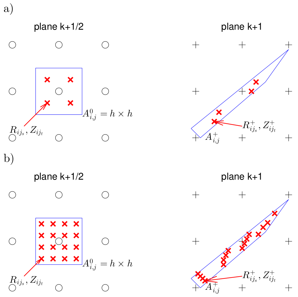
Sketch for integration via splitting into subcells for X = 1 (a) and X = 2 (b). The cross section of$A^0_{i,j}$ at plane $k+1/2$ (left) and of $A^+_{i,j}$ at plane $k+1$ (right) are illustrated. The cross section of $A^-_{i,j}$ at $k$ follows analogously.