Field line tracing and interpolation

Field line tracing

The curve along a magnetic field line, denoted as $\gamma(\varphi) = (\gamma_x, \gamma_\varphi, \gamma_y)$ is defined by the following differential equation: $$\begin{align} \dot{\gamma}(\varphi) = \begin{pmatrix} B^x/B^\varphi \\ 1\\B^y/B^\varphi\end{pmatrix}, \end{align}$$ with the initial condition: $$\begin{align} \gamma(0) = \begin{pmatrix} x_{init} \\ \varphi_{init} \\ y_{init} \end{pmatrix}, \end{align}$$

The trace routine integrates this system of equations over a toroidal distance dphi, and returns the final mapped point x_end, y_end, phi_end.

call trace(x_init, y_init, phi_init, dphi, equi, x_end, y_end, phi_end)

For numerical integration, the DOP853 ODE solver library is used, which implements a Runge-Kutta method of order 8(5,3) with step-size control.

The routine has further optional arguments:

• The length along the magnetic field line can be returned defined via the following ode: $$\begin{align} \dot{s}(\varphi) = \frac{|B(\gamma(\varphi))|}{B^\varphi(\gamma(\varphi))}, \quad \text{with}\quad s(\varphi_{init}) = 0, \end{align}$$
• The toroidal flux expansion factor, defined as: $$\begin{align} \dot{v}(\varphi) = \frac{1}{B^\varphi(\gamma(\varphi))}, \quad \text{with}\quad v(\varphi_{init}) = 0 \end{align}$$ The toroidal flux expansion is useful for accurate calculations of flux box volumes, which are required for the support operator method.
• A condition can be provided as a logical function of x, y, phi. This condition multiplies the right-hand side of the ODEs by 1 if the condition is true, or by 0 if the condition is false. This feature allows for the calculation of distances or intersection points with structures such as divertor plates or vessel walls.

Interpolation

In general, the mapped point returned by the field line tracing does not coincide with a mesh point. To obtain field values at the mapped points, 2D interpolation is performed within the adjacent poloidal planes.

The first step is to identify the interpolation stencil. For a given mapped point $x_P, y_P$​ within a plane, we need to determine which mesh points will be involved in the interpolation. For polynomial interpolation of order ns-1, where ns is an even number, the surroundingns \times ns mesh points are considered. These mesh indices can be obtained using the following mesh function:

call mesh%get_surrounding_indices(xp, yp, ns, ind_sur, ns_complete, ind_nearest)

In this call, ind_sur is a 2D array of size ns \times ns that contains the mesh indices of the surrounding points. Additionally, near boundaries, some points in the interpolation stencil may be missing. In such cases, the interpolation order is reduced. To handle this, ns_complete returns the number of complete surrounding stencil points, while ind_nearest provides the index of the nearest valid neighbor.

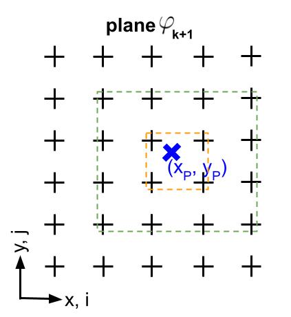
Interpolation stencil for bilinear interpolation (ns=2, orange) or 3rd order bipolynomial interpolation (ns=4, green)

For a given field $u$, where $u_l$ represents the value at mesh point $x_l, y_l$ on a specific plane, the field value at the mapped point is obtained by locally interpolating with the points surrounding the map point. This interpolation can be expressed as: $$\begin{align} u(x_P,y_P) = \sum_{i=1}^{ns}\sum_{j=1}^{ns}c_{i,j}u_{ind\_sur(i,j)}, \end{align}$$ where $c_{i,j}$ are the interpolation coefficients, which are computed using the routine interpol_coeffs routine. Since the interpolation is linear in the field values, the mapping process can also be represented as a matrix multiplication. Such a sparse matrix, which encodes the trace and interpolation, is effectively returned by the create_map_matrix routine.

As an example, the following code snippet demonstrates how to interpolate the value up from the field u using the defined interpolation procedure.

! Field
real(FP), dimension(mesh%get_n_points) :: u

! Interpolation order
integer :: intorder = 3
integer :: ns = intorder + 1 
integer, dimension(ns, ns) :: ind_sur
real(FP), dimension(ns, ns) :: coeffs

...

! Get interpolation stencil
call mesh%get_surrounding_indices(xp, yp, ns, ind_sur)

! (xrel, yrel) is coordinate w.r.t. southwest point of interpolation stencil 
! normalised to grid distance
lsw = ind_sur(1,1)
xsw = mesh%get_x(lsw)
ysw = mesh%get_y(lsw)
xrel = (xp - xsw) / mesh%get_spacing_f()
yrel = (yp - ysw) / mesh%get_spacing_f()

! Get interpolation coefficients
call interpol_coeffs(intorder, xrel, yrel, coeffs)

! Sum up interpolation from field u
up = 0.0_FP
do j = 1, ns
    do i = 1, ns
        up = up + coeffs(i, j) * u(ind_sur(i, j))
    enddo
enddo