Mesh

Initialisation and basic usage

The mesh on a given equilibrium is created using the following call:

call mesh%init(equi, phi, lvl, spacing_f, size_neighbor, size_ghost_layer)

This function generates a mesh for the specified equilibrium equi at a given toroidal angle phi, representing a two-dimensional poloidal plane (x, y). The spacing_f parameter defines the grid spacing of the mesh. The lvl parameter specifies the mesh's coarseness level, which is only needed for the multigrid preconditioner. The size_neighbor parameter controls the depth of connectivity information storage, while size_ghost_layer defines the depth of ghost points surrounding the inner mesh points. Typically, setting both size_neighbor and size_ghost_layer to 2 is recommended.

It is important to note that the mesh and any derived data is logically unstructured, meaning the locations of the grid points $x_l, y_l$ are stored as one-dimensional arrays with an index $l$. The position of the mesh points are given by: $$\begin{align} x_l = & x_{min} + (i_l-1)h, & y_l = & y_{min} + (j_l-1)h, \end{align}$$ where the fixed $x_{min}$​ and $y_{min}$ represent the coordinates of the lower-left corner of the domain​ and $h=$ spacing_f. In the code the mesh location and Cartesian grid indices can be can be accessed using getter functions:

do l = 1, mesh%get_n_points()
    x = mesh%get_x(l)
    y = mesh%get_y(l)
    i = mesh%get_cart_i(l)
    j = mesh%get_cart_j(l)
enddo

For stencil computations, the connectivity information is stored and can again be accessed using getter functions. For example, to obtain the index of the neighbor in the northwest direction, use:

l_north_west = mesh%get_index_neighbor(ishift=-1, jshift=1, ind=l)

In this example, the input parameters ishift and jshift specify the horizontal and vertical grid displacements relative to the given mesh point l, respectively. Both displacements must not exceed the value of size_neighbor. If the requested neighbor does not exist, i.e. lies outside the mesh, the function will return a value of zero.

Characterisation of mesh points

To manage boundary conditions and extended stencils, mesh points are classified into three categories:

• inner: Inner mesh points where variables are evolved according to the partial differential equations.
• boundary: Boundary points where boundary conditions are applied. These points surround the inner mesh points in both the horizontal and vertical directions and meander the continuous boundary defined by the equilibrium.
• ghost: Ghost points surround the boundary points up to a depth of size_ghost_layer. These points are useful for extending stencils beyond the physical boundary.

In the code, you can access these mesh points as follows:

! Loop over all mesh points
do l = 1, mesh%get_n_points()
    x = mesh%get_x(l) 
    ...
enddo

! Loop only over inner mesh points
do ki = 1, mesh%get_n_points_inner()
    l = mesh%inner_indices(ki)          ! Maps to global mesh index
    x = mesh%get_x(l) 
    ...
enddo

! Loop only over boundary points
do kb = 1, mesh%get_n_points_boundary()
    l = mesh%boundary_indices(kb)      ! Maps to global mesh index
    ...
enddo

! Loop only over ghost points
do kg = 1, mesh%get_n_points_boundary()
    l = mesh%ghost_indices(kg)         ! Maps to global mesh index
    ...
enddo

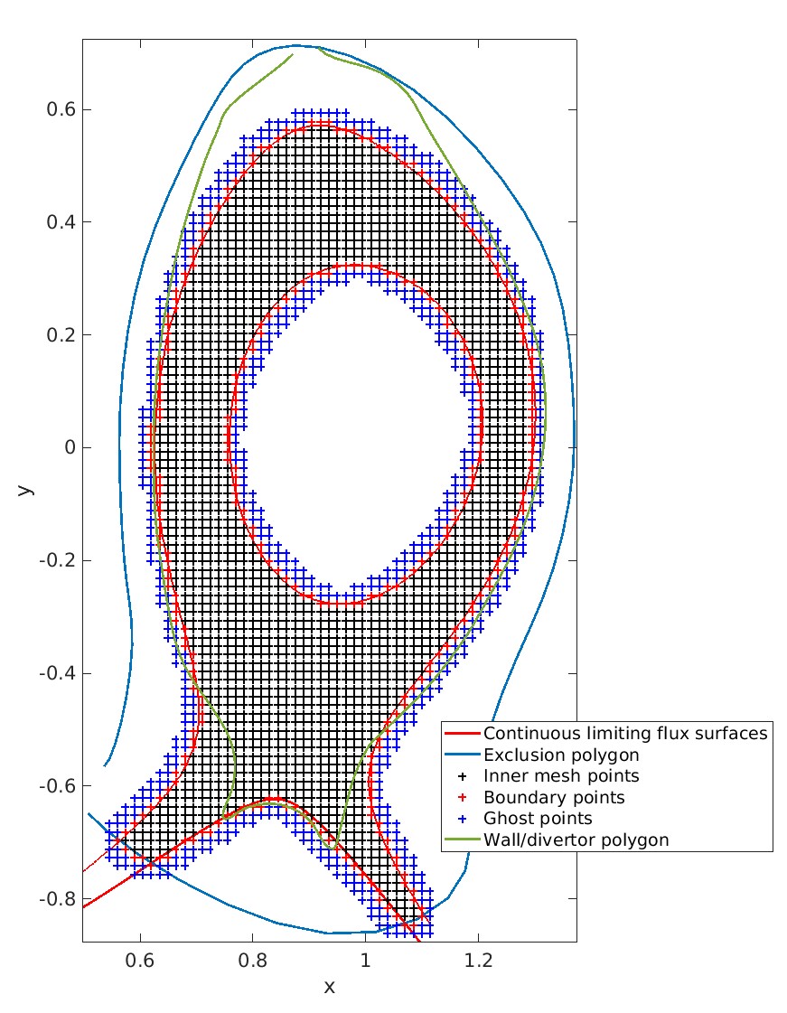Example of a mesh for a NUMERICAL equilibrium. The limiting flux surfaces (red) and the exclusion polygon (dark blue), defined by the equilibrium, form the continuous boundary. The black crosses represent inner mesh points, while the boundary points (red crosses) meander the continuous boundary. The ghost points are shown as light blue crosses. Note that the mesh may extend beyond the actual wall/divertor polygon (green) to accommodate immersed boundary condition treatment.

Districts

Further classification of mesh points based on their logical location is done using identifiers called DISTRICT:

• CLOSED: Point located within the computational domain (inner) in the closed field line region.
• SOL: Point located within the computational domain (inner) in the scrape-off layer (SOL) region.
• PRIVATE_FLUX: Point located within the computational domain (inner) in the private flux region.
• CORE: Point located outside the computational domain (boundary, ghost) beyond the inner limiting flux surface in the closed field line region.
• WALL: Point located outside the computational domain (boundary, ghost) beyond the outer limiting flux surface in the scrape-off layer region.
• DOME: Point located outside the computational domain (boundary, ghost) beyond the flux surface defining the private flux region.
• OUT: Point located outside the computational domain (boundary, ghost) within the limiting flux surfaces.

Here’s an example of how DISTRICT can be used in the code:

use descriptors_m, only : DISTRICT_CLOSED, DISTRICT_SOL
...
do l = 1, mesh%get_n_points()
    district = mesh%get_district(l)
    select case(district)
        case(DISTRICT_CLOSED)
            ! Perform operations on CLOSED points
            ...
        case(DISTRICT_SOL)
            ! Perform other operations on SOL points
            ...
        ...
    end select
enddo

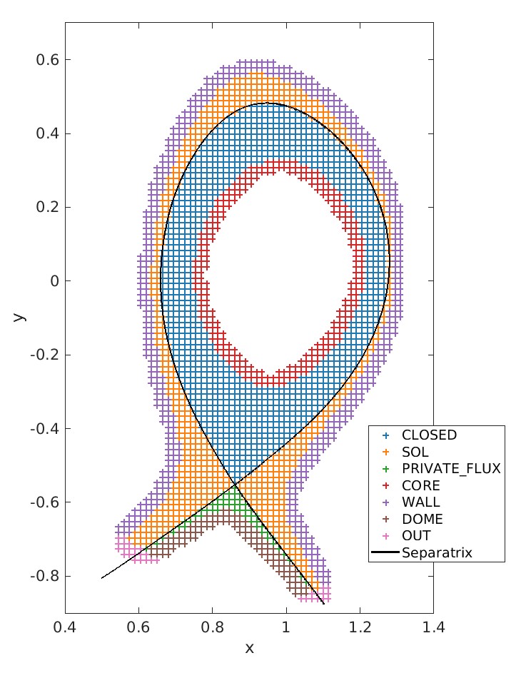
Example for the DISTRICT identifiers for a NUMERICAL diverted equilibrium.

Mesh ordering

To optimize cache efficiency, the ordering of mesh points can be arbitrarily re-shuffled after the mesh is created using the following call:

call mesh%reorder(grid_reorder_block)

The ordering strategy is determined by the grid_reorder_block parameter. Common strategies include consecutive ordering of inner, boundary, and ghost points sequentially from the lower-left to upper-right, or using an ordering based on a space-filling Z-curve.

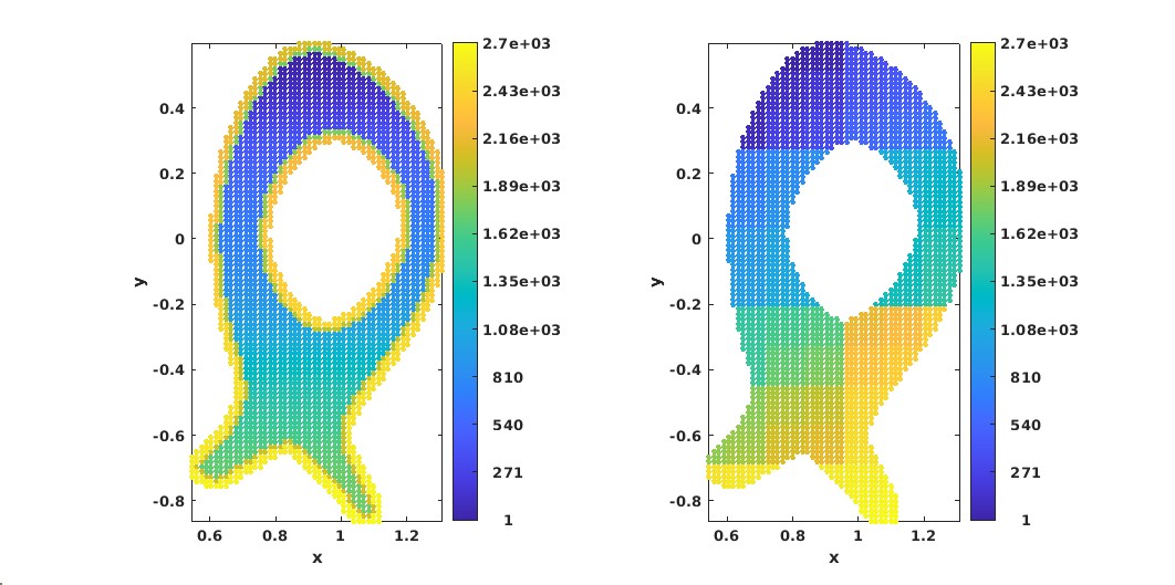
Examples for different mesh orderings. Mesh index l for consecutive ordering (left) and Morton-Z ordering (right).