Visualisation support using the VTK library
Visualization Mesh
PARALLAX offers support for 3D visualization through the VTK Fortran library. To enable this feature, you need to compile PARALLAX with the -DENABLE_VTK=ON option.
The vis_vtk3d_m module in PARALLAX computes the edges of field-aligned flux boxes centered around mesh points, along with the associated connectivity information. This data can then be written to .vtu files, which store both 2D and 3D versions of the mesh. Below is an example snippet showing how to create the 3D files:
use vtk_fortran, only : vtk_file
use vis_vtk3d_m, only : write_vtk_mesh
...
type(vtk_file) :: vtk3d
...

vtk_stat = vtk3d%initialize(format='binary', &
                            filename='vtk3d.vtu', &
                            mesh_topology='UnstructuredGrid')

! Create a locally aligned 3D mesh, with half a toroidal grid distance in both forward and backward directions
call write_vtk_mesh(equi, mesh, phi, dphi/2.0_FP, dphi/2.0_FP, vtk3d=vtk3d)

vtk_stat = vtk3d%xml_writer%write_piece()
vtk_stat = vtk3d%finalize()
The generated .vtu files can be read and visualized using tools like VisIt or ParaView.
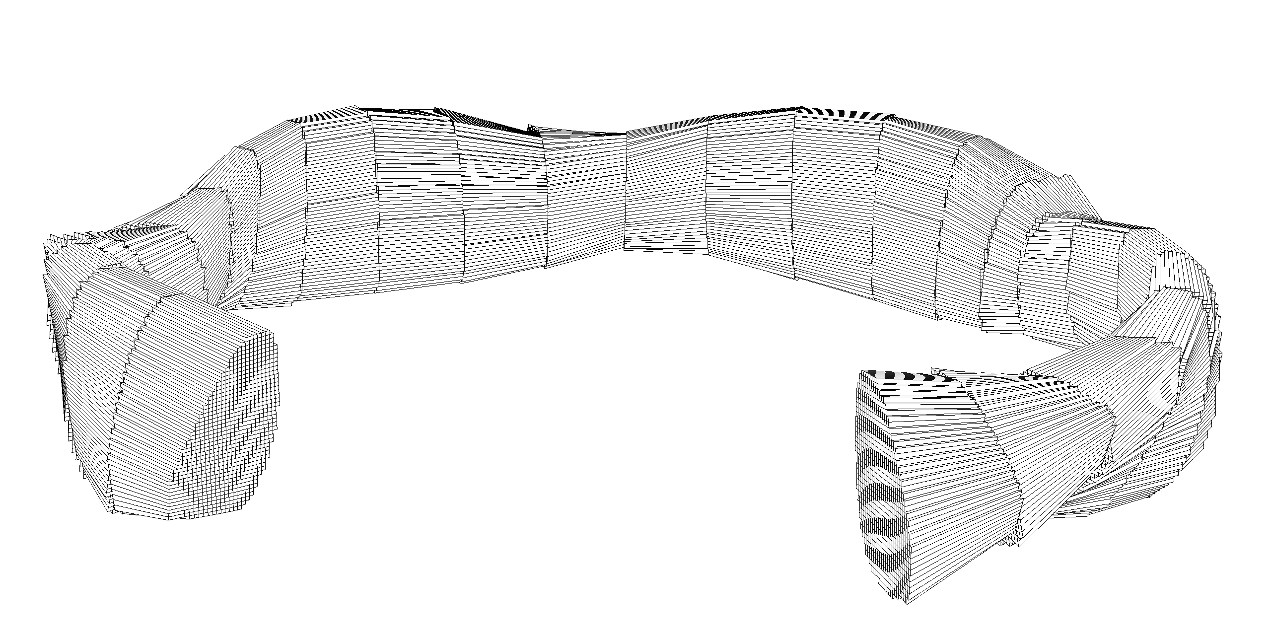
Example of a locally field-aligned mesh used for visualization in stellarator geometry. The mesh consists of locally field-aligned polyhedra, where the interface between adjacent planes is non-conformal.
Associate data with mesh
The generated .vtu yet only contain mesh information, but no simulation data. In order to associate simulation data with the mesh, a helpful little python package called meshio can be used. If you’ve already got a virtual environment for TorX, you can add this package with:
$conda activate torx
$conda install meshio -y -c conda-forge
$conda deactivate
$conda activate meshio
Below you may find a python script that then assoiates the data with the vtk mesh at the example of a GRILLIX simulation output
# This script transforms snapshot and vtk data to xdmf and h5 data
# to be used for 3D visualisation with paraview
# This script works also for 3d equilibria, but only for canonically based quantities
# Adapting the script for staggered quantities is probably not too difficult
# Usage:

# 1) conda activate torx
#    conda install meshio -y -c conda-forge
# 2) Adjust nplanes and nsnaps
# 3) Run script --> A new folder vis3d with some content should have been created
# 4) You have to move manually the data*.h files into the vis3d/ folder
# 5) Proceed with Paraview
import numpy as np
import os
import meshio
from netCDF4 import Dataset
import sys
np.set_printoptions(threshold=sys.maxsize)
p = 0

# Read plain mesh
dm = Dataset(f'trunk/multigrids_plane{p:03d}.nc')

nplanes = 25 # Number of planes, modify according to your needs
nsnaps = 86  # Number of snapshots, modify according to your needs

os.mkdir('vis3d')
for p in range(nplanes):
    print('...Processing plane', p, ' / ', nplanes-1 )
    mesh = meshio.read(f'vtk3d/vtk3d_plane{p:05d}.vtu')
    with meshio.xdmf.TimeSeriesWriter(f'vis3d/data{p:05d}.xdmf') as writer:
        writer.write_points_cells(mesh.points, mesh.cells)
        for t in range(nsnaps-1, nsnaps):
            print('.../.../Processing snaps', t+1, ' / ', nsnaps )
            # Get indices of penalisation points
            dmesh = Dataset(f'trunk/multigrids_plane{p:03d}.nc')
            inner_indices = dmesh.groups['canonical'].groups['mesh_lvl_001'].variables['inner_indices'][:]-1
            boundary_indices = dmesh.groups['canonical'].groups['mesh_lvl_001'].variables['boundary_indices'][:]-1
            ghost_indices = dmesh.groups['canonical'].groups['mesh_lvl_001'].variables['ghost_indices'][:]-1
            dpen = Dataset(f'trunk/penalisation_plane{p:03d}.nc')
            penchi = dpen.groups['canonical'].variables['charfun'][:]
            # Get simulation data
            ds = Dataset(f'snapsdir_braginskii/snaps_t{t+1:05d}.nc')
            tau = ds.variables['tau'][:]
            npoints_cano = ds.variables['npoints_cano'][:]
            npc = int(npoints_cano[p])
            ne_t = ds.variables['ne'][:]
            ne = ne_t.data[0,p,range(npc)]
            np_inner = len(inner_indices)
            # Optional: Modify data on boundaries/penalisation to NaN for clearer visualisation
            for ki in range(np_inner):
                if penchi[ki]>0.5:
                    l = inner_indices[ki]
                    ne[l] = float('NaN')
            ne[boundary_indices] = float('NaN')
            ne[ghost_indices] = float('NaN')
            # Write data
            writer.write_data(t, cell_data = dict(ne = [ne,]))
Processing the data then further via ParaView, you can then create such 3D visualisations of your simulation:
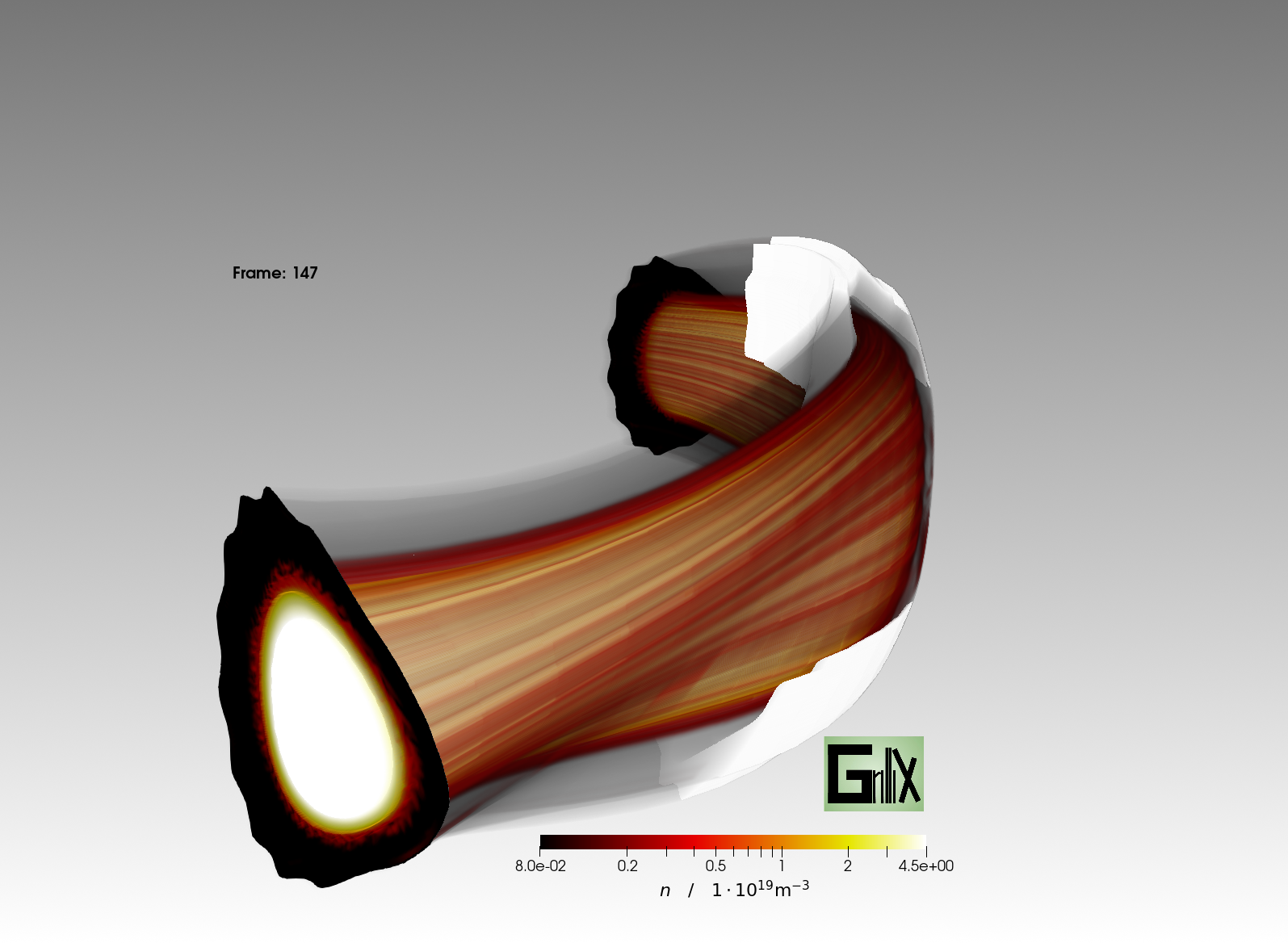
3D visualisation of a GRILLIX simulation of the W7-AS stellarator created with ParaView utilizing the NVIDIA IndeX plugin.